informatics Archives - Michael's Bioinformatics Blog

December 12, 2022December 12, 2022

MixOmics: a “swiss army knife” for -omics integration

Introduction

Genomics is the study of an organism’s complete set of genetic material, including its DNA sequence, genes, and regulation of gene expression. Other “omics” techniques, such as proteomics and metabolomics, focus on the study of proteins and metabolites, respectively. By analyzing these different types of data together, researchers can generate new insights into the inner workings of an organism and how it responds to its environment.

For example, by combining genomics data with proteomics and metabolomics data, researchers can gain a more complete understanding of an organism’s gene expression, protein production, and metabolic processes, and how these processes work together to create health, or dysfunction to create disease. This knowledge can provide valuable insights for a wide range of applications, including drug development, disease diagnosis, and environmental monitoring.

Finding correlations between related datasets means looking for patterns or relationships between different sets of data. This can provide valuable insights into the underlying biological processes and functions of an organism. For example, if two datasets show a strong positive correlation, it suggests that they are related in some way and that changes in one dataset may be associated with changes in the other. By identifying these correlations, researchers can better understand the mechanisms behind biological processes and how they are regulated. This can be useful for a variety of applications, such as predicting the effects of potential drugs or identifying potential targets for medical intervention.

I have surveyed the literature for tools to integrate multiple -omics datasets together. As is the case for any task in bioinformatics, there are dozens of options. However, when I considered criteria such as ease of installation, documentation quality, robust user community, user support and published analyses, I believe that the “mixOmics” package (available for download and installation from Bioconductor) is one of the best tools out there for doing this type of integration analysis.

The mixOmics approach

The mixOmics package encompasses many different versions of multivariate algorithms for integrating multiple datasets. Multivariate analysis is well-suited to this problem space where there are far more features than samples. By reducing the dimension of the data, the analysis makes it easier for a human analyst to see patterns and interpret correlations. One of the most common types of algorithm in mixOmics for doing this is called “partial least squares.”

Fig 1. An overview of the mixOmics package. The methods can handle single ‘omics, multiple ‘omics on the same samples (N-integration), and the same ‘omics on multiple sets of samples (P-integration) to find correlations in the data. Some examples of the graphic outputs are shown in the bottom two panels of the figure.

The partial least squares (PLS) method is a mathematical technique used to analyze relationships between two or more datasets. It works by identifying the underlying patterns and correlations in the data, and then using this information to construct a set of “composite” variables that capture the most important features of the data (this is analogous to PCA analysis, but differs by focusing on maximizing correlation/covariance among latent variables).

These composite (latent) variables can then be used to make predictions or draw conclusions about the relationships between the datasets. For example, if two datasets are known to be related in some way, the PLS method can be used to identify the specific features of each dataset that are most strongly correlated with the other, and then construct composite variables based on these features. PLS is more robust than PCA to highly correlated features and can be used to make predictions between the dependent and independent variables.

mixOmics takes the PLS method a step further by integrating a ‘feature-selection’ option called “sparse PLS” or just “sPLS” that uses “lasso” penalization to reduce unnecessary features from the final model to aid interpretation and also computational time. Lasso regression works by adding a regularization term to the ordinary least squares regression model, which is a measure of the complexity of the model. This regularization term, called the “lasso,” forces the coefficients of the model to be zero for the less important predictors, effectively eliminating them from the model.

This results in a simpler and more interpretable model that is better able to make accurate predictions. Lasso regression is particularly useful for datasets with a large number of predictors, as it can help to identify the most important predictors and reduce the risk of overfitting the model.

Conclusion

In future posts, I will describe in more detail what can be done with MixOmics and show some results from our own studies that have produced stunningly detailed and intricate correlation networks. If you are interested in this kind of work, I would encourage you to check out mixOmics as a possible avenue for analysis. There are other packages, and many of them are excellent, but the learning curve of mixOmics is quite shallow and it is well supported with a dynamic and active user community. It is also very flexible to different experimental scenarios, so that you can analyze your data several different ways while using the same package and R script.

November 18, 2014March 16, 2015

Book Review: Python for Data Analysis

Introduction

The book “Python for Data Analysis” (O’Reilly Media 2013) by author Wes McKinney is a guide to using the NumPy, matplotlib, and pandas Python libraries for data analysis. The author sets out to provide a template for Python programmers to gain working knowledge of the rapidly maturing Python technologies for data analysis and visualization tasks. The tone of the book is conversational and focused, with no fluff or filler. The book accomplishes its purpose admirably by providing a concise, meaty, and highly readable tutorial through the essential features of doing data analysis in Python.

McKinney does a skillful job of bringing the Python novice through the requisite background and quickly up to speed doing useful work with pandas without becoming bogged down in introductory Python minutia. In fact, the opening chapter is titled “Introductory Examples” and includes several relatively complex data analysis examples that serve to demonstrate the capabilities of pandas. I found this approach provided me with the motivation to read on into the more detailed and technical chapters.

Why you should listen to Wes McKinney

The author is uniquely suited to write this book, having been the creator and first developer of pandas in the course of his own work as a quantitative analyst at a hedge fund back in 2008. I could tell that the author has a mastery of the subject; he provides many useful insights that could only be gained through real-world experience. The book focuses mainly on the pandas library and its core technologies, the Series and the Dataframe. Both are important because they build on the speed and precision of numpy arrays, while allowing richer, more intuitive and powerful manipulation of data tables.

pandas: it just works the way it should

Another aspect of this book that is so enjoyable is that pandas itself just works the way I would expect it to work. The tools, in my opinion, are constructed to be as convenient and intuitive as possible. I find that pandas behaves very predictably, despite being extremely powerful. Oftentimes, I was able to invent an expression in pandas that behaved exactly as I intended without knowing a priori whether it was possible to do so. There is something very satisfying about a tool that just works and doesn’t require a lot of boilerplate code.

The publisher also provides downloadable iPython notebooks containing the code examples for each chapter. Using these notebooks it was very easy to follow along, running code while reading the chapter. The illustrations in the book also consist almost entirely of matplotlib plots prepared using the code examples. I was able to work up many of the figures, giving me a sense of having gained practical, working knowledge in each chapter.

Python for data analysis? Yes!

I really have nothing negative to say about “Python for Data Analysis”. If forced to find something to change, it would be that the author could have left out the highly-condensed chapter on introductory Python programming found at the end of the book, using the extra space instead to include even more examples of pandas in practical, real-world applications.

For instance, an example on building a data analysis model with interactive graphics for the web would have been welcome. Similarly, a demonstration of approaches for making matplotlib, with its rather utilitarian graphics, more closely resemble the stylistically attractive plots of ggplot2 (the well-known R plotting library) would also have been useful.

After reading this book, however, I have been convinced to transition my data analysis workflow entirely into Python and largely abandon R, which now seems somewhat esoteric and unnecessarily complex by comparison. Overall, I would highly recommend this book to anyone seeking to learn how to use Python for data analysis. It is a valuable reference for scientists, engineers, data analysts, and others who want to leverage the power of Python (and specifically numpy and pandas) for dealing with their data.

October 30, 2014October 30, 2014

The Python ecosystem for beginners, part 2

Welcome to Part 2 of my post on the scientific Python ecosystem (Part 1 is here). I will describe a few more of the most common and useful libraries that make up the typical Python scientific computing stack. This is not an exhaustive list by any means, and new libraries are being continually developed by the open source community.

Matplotlib – high quality 2D and 3D plotting

Matplotlib is a plotting library that aims to make it easy to produce publication quality plots. In typical Python style, Matplotlib code can be very succinct and yet yield complete, high-quality plots. The library can generate many types of 2D graphs: regular plots, histograms, scatterplots, pie charts, statistical plots, and contour plots, to name a few.

Matplotlib is organized in a hierarchical manner that allows the user to quickly and easily create plots using high-level commands, while simultaneously allowing power users to delve into the object-oriented programming layer to control minute details of individual plots, should they choose to do so.

Traits – interactive class instances and GUI building

Traits is a powerful package that extends Python type attributes in interesting and useful ways. For instance, python objects such as classes can have attribute “traits” that allow for initialization (set an default value), notification (tell another part of the program that a value has changed) and visualization (respond to GUI inputs). Although it is possible to achieve this using Python properties, Traits reduces a lot of the boilerplate code and streamlines the process.

Chaco – interactive 2D plotting

Chaco is a plotting application toolkit for building rich, interactive plots. Chaco works with Traits to build object-oriented models of plots that can accept and react to inputs from the GUI.

Cython – speed up your code with C

The easiest way to think about Cython is to imagine it as a superset of the Python language. That is, all of the normal Python language is there, along with additional commands that allow code that calls back and forth to C/C++ libraries seamlessly. In Cython, you can also add static type declarations to python functions to get C-level speedups in computation. Cython code is compiled into C code for execution. Unlike weave, which allows inline C code but requires that the python code be re-compiled for C during every execution, Cython code is compiled only once (unless there are changes later) meaning that an end user does need to bother with recompiling to run the code as a standalone program.

Using Cython for numerical computation in Python, speedups of 2000X or more above the pure Python equivalent are not uncommon.

SciKit Learn – interactive machine learning

SciKit Learn is a machine-learning library for Python. It is based on NumPy, SciPy and matplotlib. There are many algorithms available for performing machine-learning tasks, falling into four main areas: classification, clustering, regression, and dimensionality reduction (principle component analysis).

October 22, 2014October 30, 2014

The Python ecosystem for beginners

When first starting to learn Python, I found the array of package names and libraries a bit bewildering and confusing. In this post I will enumerate many of the most common and useful parts of the Python computing “ecosystem” and attempt to describe them very briefly.

My aim is to provide some clarity on the situation for new users, as I would have liked to have seen the “30,000 ft view” when I started learning not long ago. So without further ado, part 1 of the python ecosystem overview:

Python -high-level, interpreted language

Python is an interpreted programming language (itself written in C) that allows you to write very clean and simple code in a fast and human-readable form as compared to lower-level compiled languages (C++, Fortran).

The language is simple, self-consistent and beautiful. It is relatively easy to learn and is gaining in popularity every year. The simplicity and ease of use does come with a price as code written in pure Python is generally slower to execute than compiled C/C++ code.

iPython -get code written faster

iPython is an enhanced, interactive Python shell designed to make code development faster. According to Wes McKinney in his excellent book, “Python for Data Analysis,” iPython is designed to encourage “an execute-explore workflow instead of the typical edit-compile-run workflow of many other programming languages.”

iPython contains the Python interpreter and is ready to execute commands as you enter them. It is where you run code snippets, examine the outputs, and make iterative improvements. In that sense, it is like kind of like the UNIX command line. You don’t write full programs here, you do that in a text editor or IDE (integrated development environment).

It also contains useful features called “magic commands.” These are commands that are unique to the iPython command line, and are not valid Python code (i.e., you cannot use these commands in stand-alone programs). Magic commands provide productivity speedups in many useful ways, such as recalling command history, running parts of scripts, timing code, and debugging code interactively.

If you have iPython installed you can invoke it from a regular python shell; however I find it easiest to use it within an IDE that supports iPython.

iPython Notebook -share code and ideas over the web

The iPython notebook is an interactive python format that runs in a web browser or in an IDE. The Notebook is a flexible and powerful document format that allows python code, text markdown, mathematics equations, and figures to be displayed together in a coherent, inline way. An iPython notebook could be used to provide all of the steps in a data analysis project, for example, or to teach a programming concept. It is very useful for sharing code and visualizing results in an interactive, portable document.

NumPy -implement very fast vectorized computation

NumPy (numerical python) is a powerful and fast library for doing numerical computation in Python. It is based on a data structure called an ndarray. This lower level structure is faster for computation than regular higher-level python structures like lists and dictionaries, but it is less flexible and behaves in somewhat unintuitive ways. Functions can be applied across a numpy array all at once and “in place”; this is known as vectorization. NumPy contains a number of vectorized built-in functions known as “ufuncs” for doing transformations on ndarrrays.

pandas -powerful library for data analysis

pandas is a data analysis package for python; conceived and built initially by Wes McKinney. It was developed to allow python users to access some of the powerful features of the R statistics language while staying in the python ecosystem. Prior to the development of pandas, data analysis had to be carried out using the NumPy ndarray structures which are rather difficult for handling messy real world data.

Pandas achieves very fast speeds and efficiency because it is built on top of NumPy and therefore takes advantage of the built-in speed advantage of the low-level ndarray data structures. However, pandas allows users to create higher-level structures called Series (1D), Dataframes (2D) and Panels (3D), that are more flexible and useful for regular data analysis than raw numpy arrays owing to their ability to contain mixed data types, headers, and indexes.

Pandas also contains many built-in methods for operations on Series, Dataframes, and Panels that allow users to quickly and easily do data aggregation, reductions, and “split-apply-combine” strategies.

SciPy -collection of libraries for a variety of computing applications

SciPy is a collection of scientific algorithms for doing scientific computing. It is an open-source project under active development. Some of the packages available include scipy.linalg for doing linear algebra, scipy.stats for statistics, scipy.cluster for clustering (K-means and others), scipy.fftpack for doing fourier transform analysis, scipy.optimize for doing curve fitting and minimization, and scipy.signal for doing signal processing. There are many more packages in SciPy; what you end up using will depend on your application and area of interest.

In part 2, I will describe even more libraries and packages that you will encounter as you learn scientific computing with Python.

August 7, 2014March 16, 2015

What is tidy data?

What is “tidy” data?

What is meant by the term “tidy” data, as opposed to “messy” data? In my last post I listed five of the most common problems encountered with messy datasets. Logically, “tidy” data must not have any of these problems. So just what does tidy data look like?

Let’s take a look at an example of tidy data. Below are the first 20 lines from R’s built-in “airquality” dataset:

Fig 1. Air quality dataset is messy data. — Figure 1. The “airquality” dataset.

According to R programmer and professor of statistics Hadley Wickham, tidy data can be defined as the following:

1) Each variable forms a column

2) Each observation forms a row

3) Each type of observational unit forms a table

That’s it. “Airquality” is tidy because each row corresponds to one month/day combination and the four measured weather variables (ozone, solar, wind, and temp) on that day.

What about messy data?

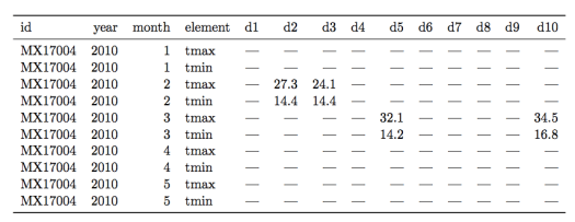
Let’s see an example of a messy weather dataset for a counterexample (data examples are from this paper by H. Wickham):

Figure 2. A messy weather dataset. Not all columns are shown for the sake of clarity. — Figure 2. A messy weather station dataset. Not all columns are shown for the sake of clarity.

There are multiple “messy” data problems with this table. First, identifying variables like day of the month are stored in column headers (“d1”, “d2”, etc…), not in rows. Second, there are a lot of missing values, complicating analysis and making it harder to read the table. Third, the column “element” consists of variable names (“tmin” and “tmax”) violating rule 1 of tidy data.

How to use R tools to transform this table into tidy form is beyond the scope of this post, so I will just show the tidy version of this dataset in Figure 3.

Screen shot 2014-08-01 at 1.55.23 PM — Figure 3. The weather station data in tidy form.

Each column now forms a unique variable. The date information has been condensed into a more compact form and each row contains the measurements for only one day. The two variables in the “element” column are now forming their own columns, “tmax” and “tmin.” With the data in this form it is far easier to prepare plots, aggregate the data, and perform statistical analysis.